The Illustrated Transformer

介绍

本文是The Illustrated Transformer原文与译文。

引言

In the previous post, we looked at Attention – a ubiquitous method in modern deep learning models. Attention is a concept that helped improve the performance of neural machine translation applications. In this post, we will look at The Transformer – a model that uses attention to boost the speed with which these models can be trained. The Transformer outperforms the Google Neural Machine Translation model in specific tasks. The biggest benefit, however, comes from how The Transformer lends itself to parallelization. It is in fact Google Cloud’s recommendation to use The Transformer as a reference model to use their Cloud TPU offering. So let’s try to break the model apart and look at how it functions.

在上一篇文章中，我们了解了 Attention——这是一种在现代深度学习模型中普遍使用的方法。Attention 是一个帮助提高神经机器翻译应用性能的概念。在这篇文章中，我们将探讨 The Transformer——一个使用 Attention 来提高这些模型训练速度的模型。The Transformer 在特定任务中优于 Google 神经机器翻译模型。然而，最大的好处来自于 The Transformer 如何便于并行化。事实上，Google Cloud 推荐使用 The Transformer 作为参考模型来使用他们的 Cloud TPU 服务。所以让我们尝试将模型分解开来，看看它是如何运作的。

The Transformer was proposed in the paper Attention is All You Need. A TensorFlow implementation of it is available as a part of the Tensor2Tensor package. Harvard’s NLP group created a guide annotating the paper with PyTorch implementation. In this post, we will attempt to oversimplify things a bit and introduce the concepts one by one to hopefully make it easier to understand to people without in-depth knowledge of the subject matter.

Transformer 模型是在论文《Attention is All You Need》中提出的。它的 TensorFlow 实现作为 Tensor2Tensor 包的一部分提供。哈佛大学自然语言处理小组创建了一份指南，用 PyTorch 实现标注了这篇论文。在这篇文章中，我们将尝试简化一些内容，逐一介绍这些概念，希望能让那些对主题没有深入知识的人更容易理解。

A High-Level Look 高层视角

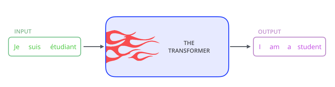
Let’s begin by looking at the model as a single black box. In a machine translation application, it would take a sentence in one language, and output its translation in another.

让我们从一个黑盒的角度来观察这个模型。在机器翻译应用中，它会输入一种语言的句子，并输出其翻译到另一种语言。

Popping open that Optimus Prime goodness, we see an encoding component, a decoding component, and connections between them.

打开那个擎天柱的精华，我们看到一个编码组件、一个解码组件以及它们之间的连接。

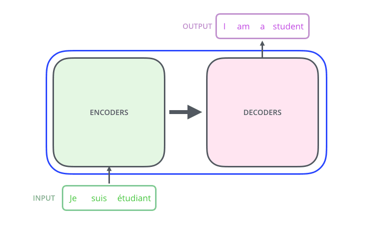
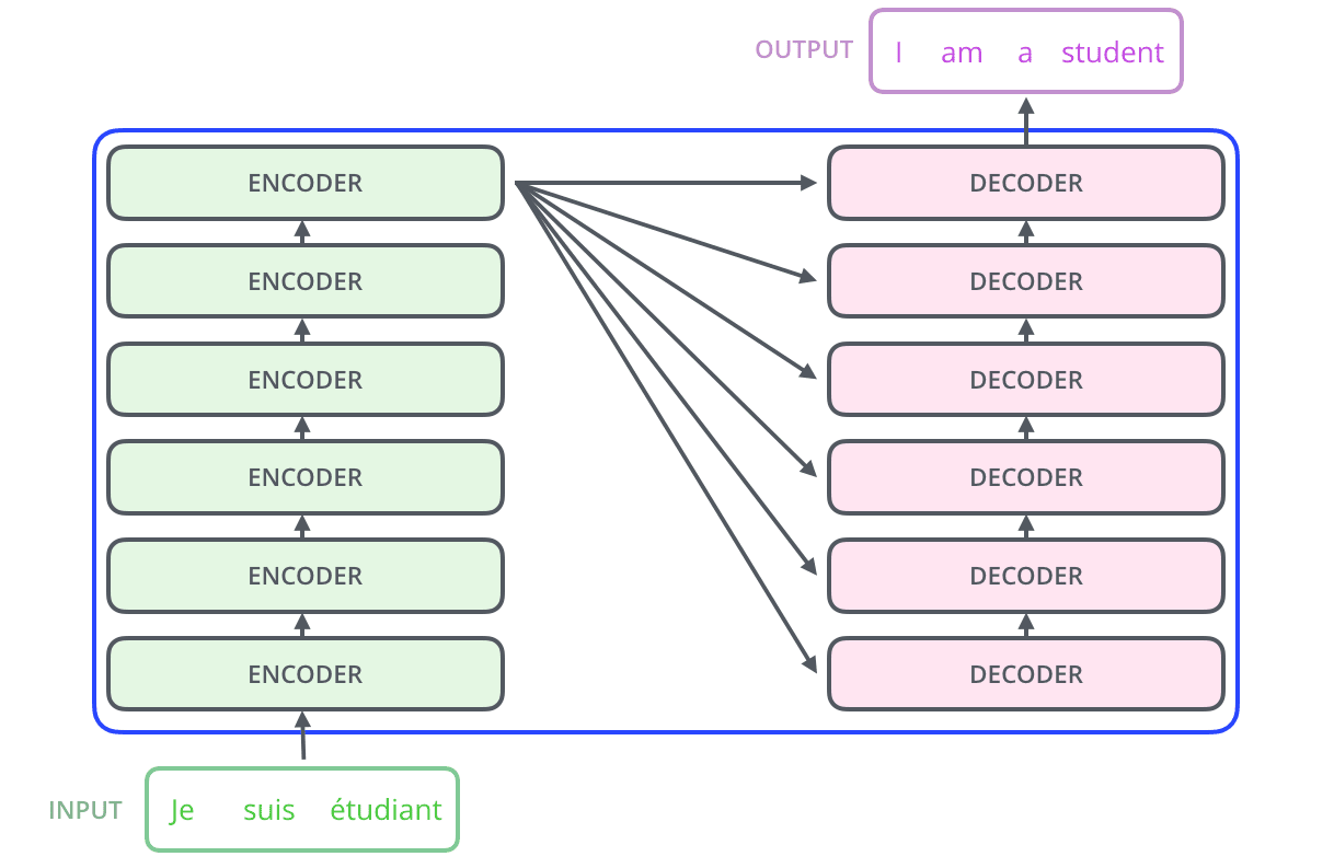
The encoding component is a stack of encoders (the paper stacks six of them on top of each other – there’s nothing magical about the number six, one can definitely experiment with other arrangements). The decoding component is a stack of decoders of the same number.

编码组件是一叠编码器（论文将六个编码器叠在一起——六这个数字没什么神奇之处，完全可以尝试其他排列方式）。解码组件是相同数量的解码器叠在一起。

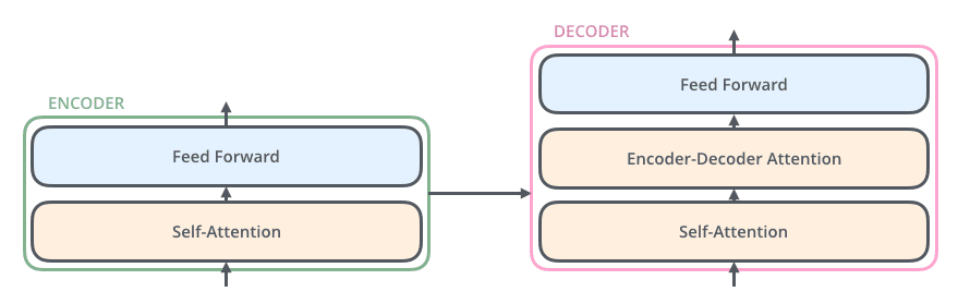
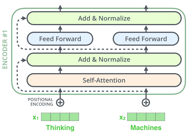
The encoders are all identical in structure (yet they do not share weights). Each one is broken down into two sub-layers:

编码器在结构上完全相同（但它们不共享权重）。每个编码器被分解为两个子层：

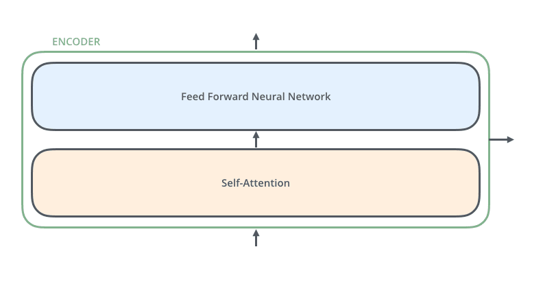
The encoder’s inputs first flow through a self-attention layer – a layer that helps the encoder look at other words in the input sentence as it encodes a specific word. We’ll look closer at self-attention later in the post.

编码器的输入首先流经一个自注意力层——一个帮助编码器在编码特定单词时查看输入句子中其他单词的层。我们将在本文稍后更详细地探讨自注意力。

The outputs of the self-attention layer are fed to a feed-forward neural network. The exact same feed-forward network is independently applied to each position.

自注意力层的输出被输入到一个前馈神经网络。完全相同的前馈网络独立地应用于每个位置。

The decoder has both those layers, but between them is an attention layer that helps the decoder focus on relevant parts of the input sentence (similar what attention does in seq2seq models).

解码器包含这两层，但在它们之间有一个注意力层，帮助解码器关注输入句子的相关部分（类似于注意力在 seq2seq 模型中的作用）。

Bringing The Tensors Into The Picture 将张量引入画面

Now that we’ve seen the major components of the model, let’s start to look at the various vectors/tensors and how they flow between these components to turn the input of a trained model into an output.

现在我们已经了解了模型的主要组件，让我们开始查看各种向量/张量以及它们如何在这些组件之间流动，以将训练模型的输入转换为输出。

As is the case in NLP applications in general, we begin by turning each input word into a vector using an embedding algorithm.

与 NLP 应用的一般情况一样，我们首先使用嵌入算法将每个输入词转换为向量。

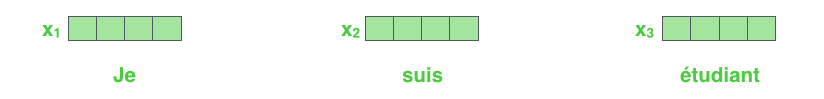
Each word is embedded into a vector of size 512. We'll represent those vectors with these simple boxes.

每个词被嵌入到一个大小为 512 的向量中。我们将用这些简单的方框来表示这些向量。

The embedding only happens in the bottom-most encoder. The abstraction that is common to all the encoders is that they receive a list of vectors each of the size 512 – In the bottom encoder that would be the word embeddings, but in other encoders, it would be the output of the encoder that’s directly below. The size of this list is hyperparameter we can set – basically it would be the length of the longest sentence in our training dataset.

嵌入只在最底层的编码器中发生。所有编码器共有的抽象概念是它们接收一个由 512 维向量组成的列表——在最底层的编码器中，这将是词嵌入，但在其他编码器中，它将是直接位于其下方的编码器的输出。这个列表的大小是一个我们可以设置的超参数——基本上，它将是我们的训练数据集中最长句子的长度。

After embedding the words in our input sequence, each of them flows through each of the two layers of the encoder.

在将输入序列中的词嵌入后，每个词都会通过编码器的两个层。

Here we begin to see one key property of the Transformer, which is that the word in each position flows through its own path in the encoder. There are dependencies between these paths in the self-attention layer. The feed-forward layer does not have those dependencies, however, and thus the various paths can be executed in parallel while flowing through the feed-forward layer.

从这里我们可以看到 Transformer 的一个关键特性，即每个位置中的词在编码器中通过自己的路径流动。在这些路径之间存在自注意力层之间的依赖关系。然而，前馈层没有这些依赖关系，因此各种路径可以在通过前馈层时并行执行。

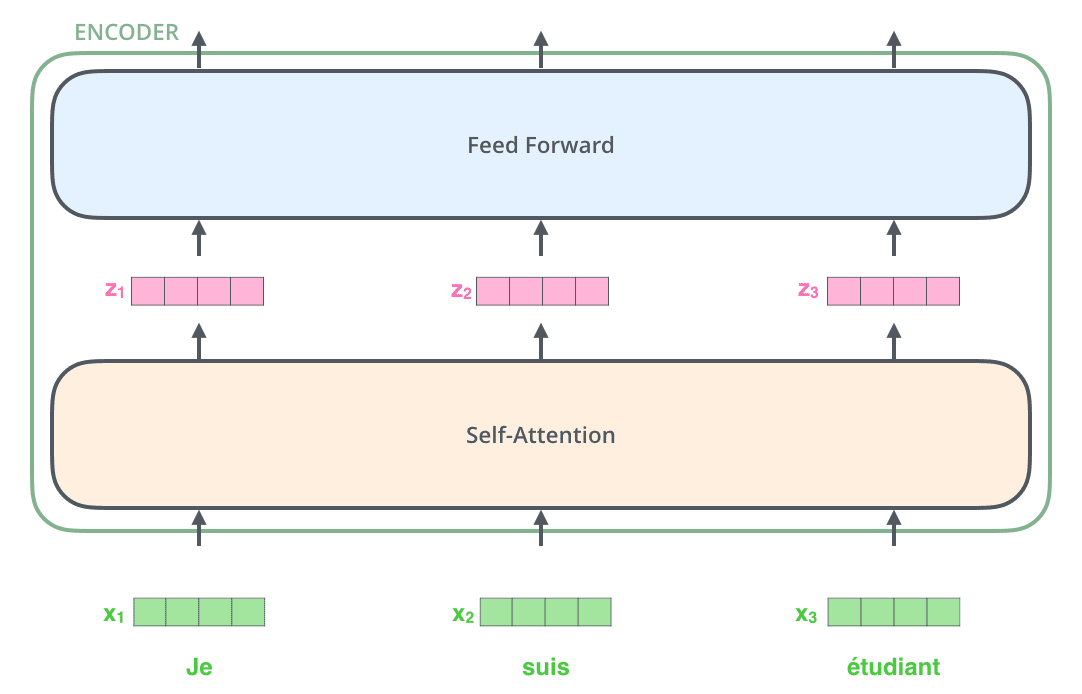
Next, we’ll switch up the example to a shorter sentence and we’ll look at what happens in each sub-layer of the encoder.

接下来，我们将示例改为一个更短的句子，并查看编码器每个子层中的情况。

Now We’re Encoding! 现在我们开始编码

As we’ve mentioned already, an encoder receives a list of vectors as input. It processes this list by passing these vectors into a ‘self-attention’ layer, then into a feed-forward neural network, then sends out the output upwards to the next encoder.

正如我们之前提到的，编码器接收一个向量列表作为输入。它通过将这些向量传递到“自注意力”层，然后传递到前馈神经网络，然后将输出向上发送到下一个编码器。

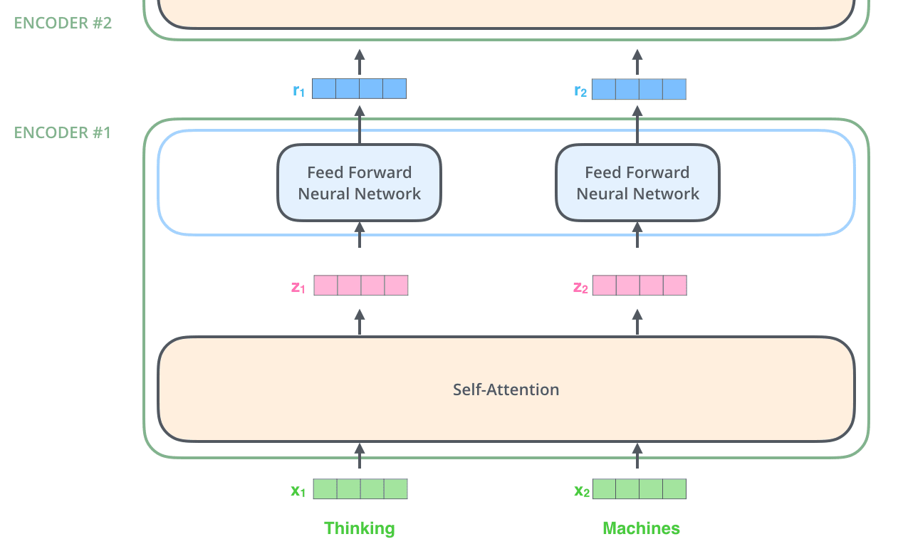
The word at each position passes through a self-attention process. Then, they each pass through a feed-forward neural network -- the exact same network with each vector flowing through it separately.

每个位置的词会经过自注意力处理。然后，它们各自会通过一个前馈神经网络——每个向量都单独流经同一个网络。

Self-Attention at a High Level 自注意力高层概述

Don’t be fooled by me throwing around the word “self-attention” like it’s a concept everyone should be familiar with. I had personally never came across the concept until reading the Attention is All You Need paper. Let us distill how it works.

不要被我用“自注意力”这个词来误导，好像这是每个人都应该熟悉的概念。我本人直到读到《Attention is All You Need》这篇论文之前，都没遇到过这个概念。让我们提炼一下它是如何工作的。

Say the following sentence is an input sentence we want to translate:

假设以下句子是我们想要翻译的输入句子：

”The animal didn't cross the street because it was too tired”

What does “it” in this sentence refer to? Is it referring to the street or to the animal? It’s a simple question to a human, but not as simple to an algorithm.

这句话中的“it”指的是什么？是指街道还是指动物？对人类来说这是个简单的问题，但对算法来说就不那么简单了。

When the model is processing the word “it”, self-attention allows it to associate “it” with “animal”.

当模型处理单词“it”时，自注意力机制允许它将“it”与“animal”联系起来。

As the model processes each word (each position in the input sequence), self attention allows it to look at other positions in the input sequence for clues that can help lead to a better encoding for this word.

随着模型处理每个单词（输入序列中的每个位置），自注意力机制允许它查看输入序列中的其他位置，以寻找有助于为这个单词提供更好的编码的线索。

If you’re familiar with RNNs, think of how maintaining a hidden state allows an RNN to incorporate its representation of previous words/vectors it has processed with the current one it’s processing. Self-attention is the method the Transformer uses to bake the “understanding” of other relevant words into the one we’re currently processing.

如果你熟悉 RNN，可以想象如何通过维护隐藏状态使 RNN 能够将已处理的前一个词/向量的表示与当前正在处理的词结合起来。自注意力机制是 Transformer 用来将其他相关词的“理解”嵌入到当前正在处理的词中的方法。

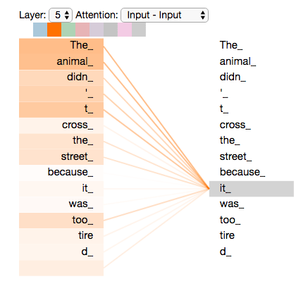
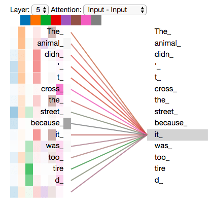
As we are encoding the word "it" in encoder #5 (the top encoder in the stack), part of the attention mechanism was focusing on "The Animal", and baked a part of its representation into the encoding of "it".

当我们正在对堆栈顶部的编码器#5 编码单词"it"时，注意力机制的一部分专注于"The Animal"，并将其部分表示嵌入到"it"的编码中。

Be sure to check out the Tensor2Tensor notebook where you can load a Transformer model, and examine it using this interactive visualization.

请务必查看 Tensor2Tensor 笔记本，在那里你可以加载一个 Transformer 模型，并使用这个交互式可视化来检查它。

Self-Attention in Detail 自注意力机制详解

Let’s first look at how to calculate self-attention using vectors, then proceed to look at how it’s actually implemented – using matrices.

让我们首先看看如何使用向量计算自注意力，然后继续探讨其实际实现——使用矩阵。

The first step in calculating self-attention is to create three vectors from each of the encoder’s input vectors (in this case, the embedding of each word). So for each word, we create a Query vector, a Key vector, and a Value vector. These vectors are created by multiplying the embedding by three matrices that we trained during the training process.

计算自注意力的第一步是从编码器的每个输入向量（在这种情况下，每个单词的嵌入）中创建三个向量。因此，对于每个单词，我们创建一个查询向量、一个键向量和一个值向量。这些向量是通过将嵌入乘以在训练过程中训练的三个矩阵来创建的。

Notice that these new vectors are smaller in dimension than the embedding vector. Their dimensionality is 64, while the embedding and encoder input/output vectors have dimensionality of 512. They don’t HAVE to be smaller, this is an architecture choice to make the computation of multiheaded attention (mostly) constant.

请注意，这些新向量的维度比嵌入向量小。它们的维度是 64，而嵌入和编码器输入/输出向量的维度是 512。它们不必更小，这是一个架构选择，以使多头注意力的计算（主要）保持恒定。

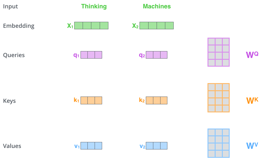
Multiplying x1 by the WQ weight matrix produces q1, the "query" vector associated with that word. We end up creating a "query", a "key", and a "value" projection of each word in the input sentence.

将 x1 乘以 WQ 权重矩阵产生 q1，与该单词相关的“查询”向量。我们最终为输入句子中的每个单词创建了一个“查询”、一个“键”和一个“值”投影。

What are the “query”, “key”, and “value” vectors?

“查询”、“键”和“值”向量是什么？

They’re abstractions that are useful for calculating and thinking about attention. Once you proceed with reading how attention is calculated below, you’ll know pretty much all you need to know about the role each of these vectors plays.

它们是用于计算和思考注意力的抽象概念。一旦你继续阅读下面关于注意力如何计算的说明，你就会知道关于每个向量所起作用的所有必要信息。

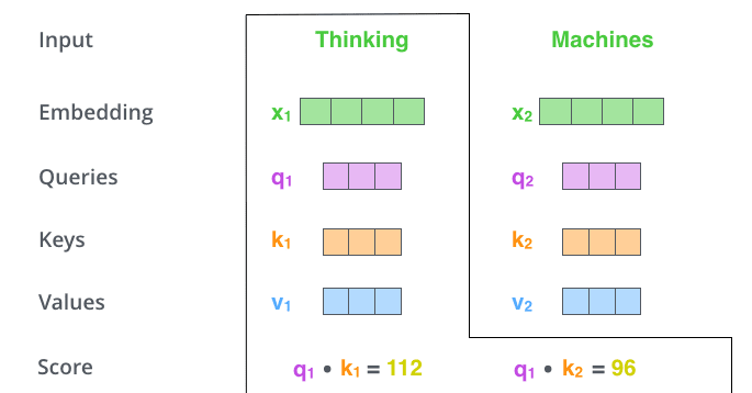
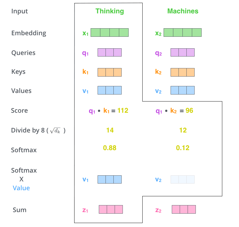
The second step in calculating self-attention is to calculate a score. Say we’re calculating the self-attention for the first word in this example, “Thinking”. We need to score each word of the input sentence against this word. The score determines how much focus to place on other parts of the input sentence as we encode a word at a certain position.

计算自注意力过程的第二步是计算一个分数。假设我们正在计算这个例子中第一个词“Thinking”的自注意力。我们需要将输入句子的每个词与这个词进行评分。这个分数决定了在编码某个位置的词时，应该将多少注意力放在输入句子的其他部分上。

The score is calculated by taking the dot product of the query vector with the key vector of the respective word we’re scoring. So if we’re processing the self-attention for the word in position #1, the first score would be the dot product of q1 and k1. The second score would be the dot product of q1 and k2.

该分数是通过将查询向量与我们要评分的相应词的键向量进行点积计算得出的。所以，如果我们正在处理位置#1 的词的自注意力，第一个分数将是 q1 和 k1 的点积。第二个分数将是 q1 和 k2 的点积。

The third and fourth steps are to divide the scores by 8 (the square root of the dimension of the key vectors used in the paper – 64. This leads to having more stable gradients. There could be other possible values here, but this is the default), then pass the result through a softmax operation. Softmax normalizes the scores so they’re all positive and add up to 1.

第三步和第四步是将分数除以 8（论文中使用的键向量的维度的平方根——64。这会导致梯度更加稳定。这里可能有其他可能的值，但这是默认值），然后将结果通过 softmax 操作。Softmax 将分数归一化，使它们都是正数并且总和为 1。

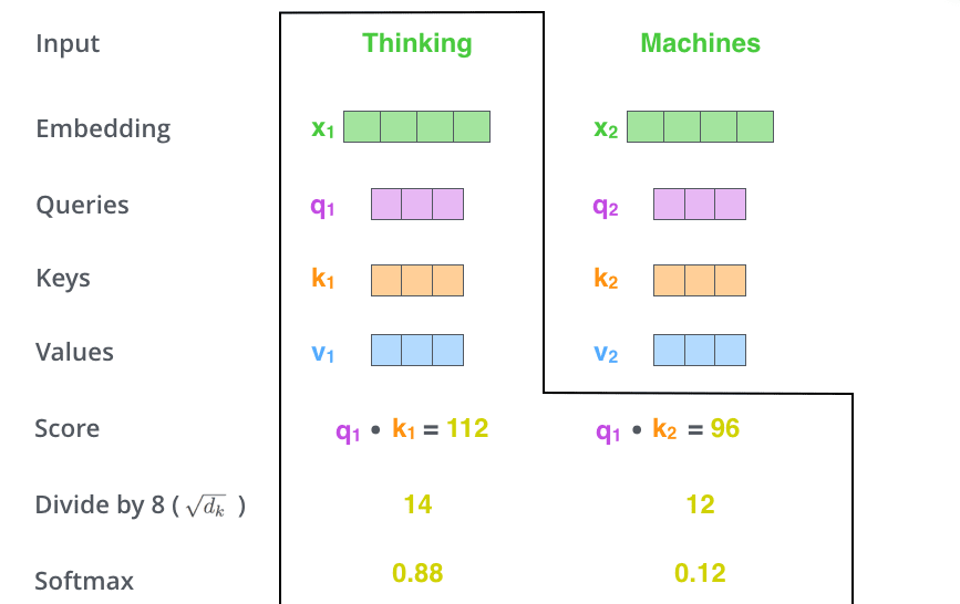
This softmax score determines how much each word will be expressed at this position. Clearly the word at this position will have the highest softmax score, but sometimes it’s useful to attend to another word that is relevant to the current word.

这个 softmax 分数决定了每个词在这个位置上的表达程度。显然，这个位置的词将拥有最高的 softmax 分数，但有时关注与当前词相关的另一个词也是有用的。

The fifth step is to multiply each value vector by the softmax score (in preparation to sum them up). The intuition here is to keep intact the values of the word(s) we want to focus on, and drown-out irrelevant words (by multiplying them by tiny numbers like 0.001, for example).

第五步是将每个值向量乘以 softmax 分数（为求和做准备）。这里的直觉是保持我们想要关注的词的值不变，通过乘以很小的数（例如 0.001）来抑制无关的词。

The sixth step is to sum up the weighted value vectors. This produces the output of the self-attention layer at this position (for the first word).

第六步是求和加权后的值向量。这产生了自注意力层在这个位置（对于第一个词）的输出。

That concludes the self-attention calculation. The resulting vector is one we can send along to the feed-forward neural network. In the actual implementation, however, this calculation is done in matrix form for faster processing. So let’s look at that now that we’ve seen the intuition of the calculation on the word level.

自注意力计算到此结束。这个结果向量可以传递给前馈神经网络。然而，在实际实现中，这个计算是以矩阵形式进行的，以便更快地处理。现在我们已经了解了单词层面的计算直觉，让我们来看看矩阵形式的计算。

Matrix Calculation of Self-Attention 自注意力矩阵计算

The first step is to calculate the Query, Key, and Value matrices. We do that by packing our embeddings into a matrix X, and multiplying it by the weight matrices we’ve trained (WQ, WK, WV).

第一步是计算查询、键和值矩阵。我们通过将嵌入打包到矩阵 X 中，并将其乘以我们训练的权重矩阵（WQ、WK、WV）来完成这一步。

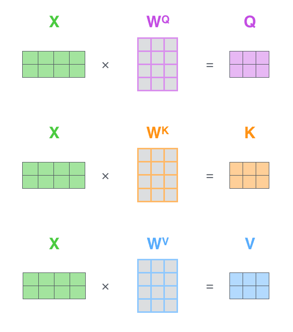
Every row in the X matrix corresponds to a word in the input sentence. We again see the difference in size of the embedding vector (512, or 4 boxes in the figure), and the q/k/v vectors (64, or 3 boxes in the figure)

X 矩阵中的每一行对应输入句子中的一个词。我们再次看到嵌入向量的大小差异（512，或图中 4 个方框），以及 q/k/v 向量的大小（64，或图中 3 个方框）。

Finally, since we’re dealing with matrices, we can condense steps two through six in one formula to calculate the outputs of the self-attention layer.

最后，由于我们处理的是矩阵，可以将步骤二至步骤六合并为一个公式来计算自注意力层的输出。

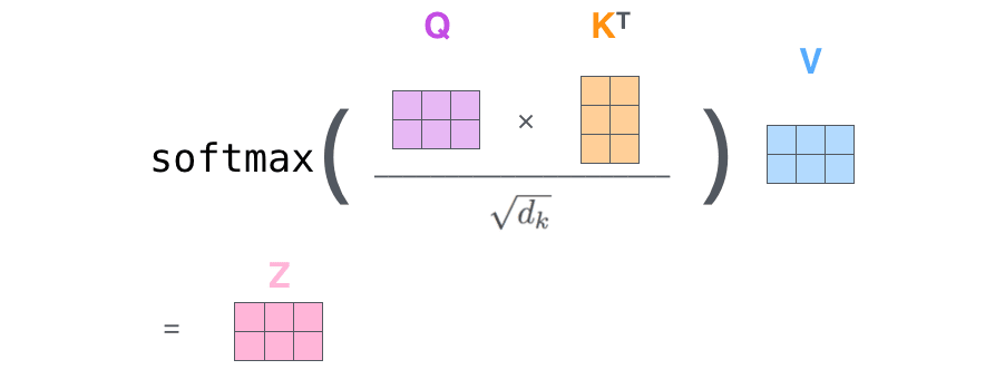
The self-attention calculation in matrix form

矩阵形式的自我注意力计算

The Beast With Many Heads 多头怪兽

The paper further refined the self-attention layer by adding a mechanism called “multi-headed” attention. This improves the performance of the attention layer in two ways:

论文进一步通过引入“多头”注意力机制来优化自注意力层。这种改进在两个方面提升了注意力层的性能：

• It expands the model’s ability to focus on different positions. Yes, in the example above, z1 contains a little bit of every other encoding, but it could be dominated by the actual word itself. If we’re translating a sentence like “The animal didn’t cross the street because it was too tired”, it would be useful to know which word “it” refers to.

• 它扩展了模型对不同位置的关注能力。是的，在上面的例子中，z1 包含了每个编码的一小部分，但它可能被实际单词本身主导。如果我们正在翻译像“动物没有穿过街道，因为它太累了”这样的句子，知道“it”指的是哪个词会很有用。

• It gives the attention layer multiple “representation subspaces”. As we’ll see next, with multi-headed attention we have not only one, but multiple sets of Query/Key/Value weight matrices (the Transformer uses eight attention heads, so we end up with eight sets for each encoder/decoder). Each of these sets is randomly initialized. Then, after training, each set is used to project the input embeddings (or vectors from lower encoders/decoders) into a different representation subspace.

• 它为注意力层提供了多个“表示子空间”。接下来我们将看到，通过多头注意力机制，我们不仅有一个，而是有多个查询/键/值权重矩阵（Transformer 使用八个注意力头，因此每个编码器/解码器最终都会有八个这样的集合）。这些集合都是随机初始化的。然后，在训练后，每个集合都会将输入嵌入（或来自较低编码器/解码器的向量）投影到不同的表示子空间中。

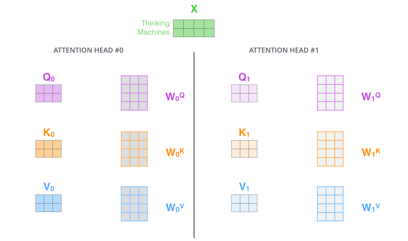
With multi-headed attention, we maintain separate Q/K/V weight matrices for each head resulting in different Q/K/V matrices. As we did before, we multiply X by the WQ/WK/WV matrices to produce Q/K/V matrices.

通过多头注意力机制，我们为每个注意力头维护独立的 Q/K/V 权重矩阵，从而产生不同的 Q/K/V 矩阵。与之前一样，我们将 X 乘以 WQ/WK/WV 矩阵，以生成 Q/K/V 矩阵。

If we do the same self-attention calculation we outlined above, just eight different times with different weight matrices, we end up with eight different Z matrices

如果我们按照上面概述的相同自注意力计算方法，只是用不同的权重矩阵重复进行八次，最终我们会得到八个不同的 Z 矩阵

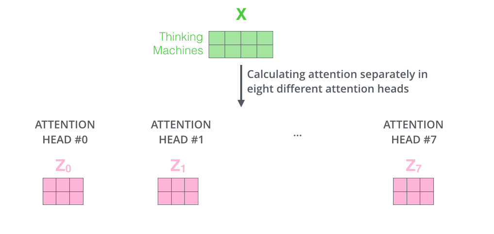
This leaves us with a bit of a challenge. The feed-forward layer is not expecting eight matrices – it’s expecting a single matrix (a vector for each word). So we need a way to condense these eight down into a single matrix.

这给我们带来了一些挑战。前馈层不是期望八个矩阵——它期望一个单一的矩阵（每个词一个向量）。所以我们需要一种方法将这些八个矩阵压缩成一个矩阵。

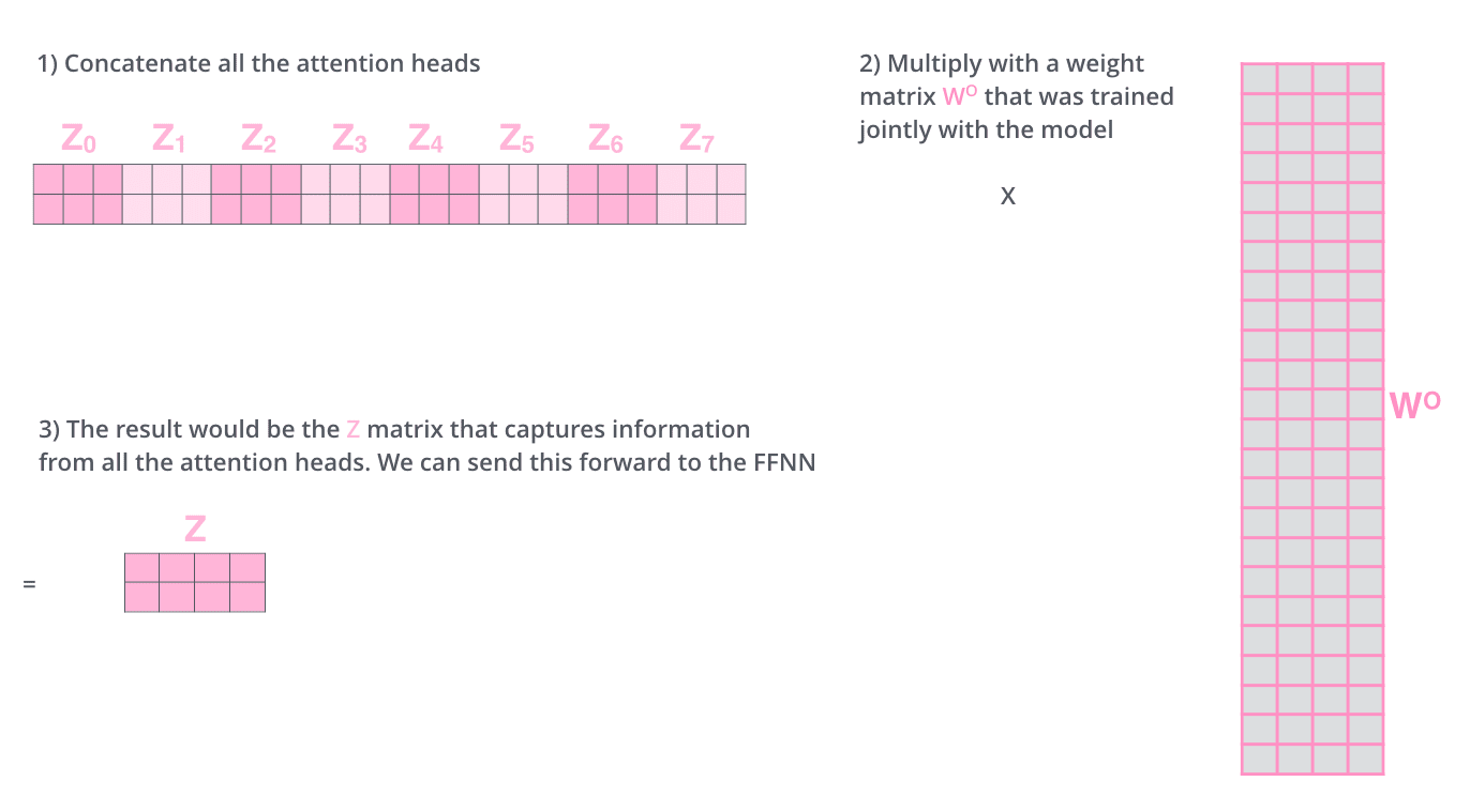
How do we do that? We concat the matrices then multiply them by an additional weights matrix WO.

我们该如何做到呢？我们将这些矩阵连接起来，然后乘以一个额外的权重矩阵 WO。

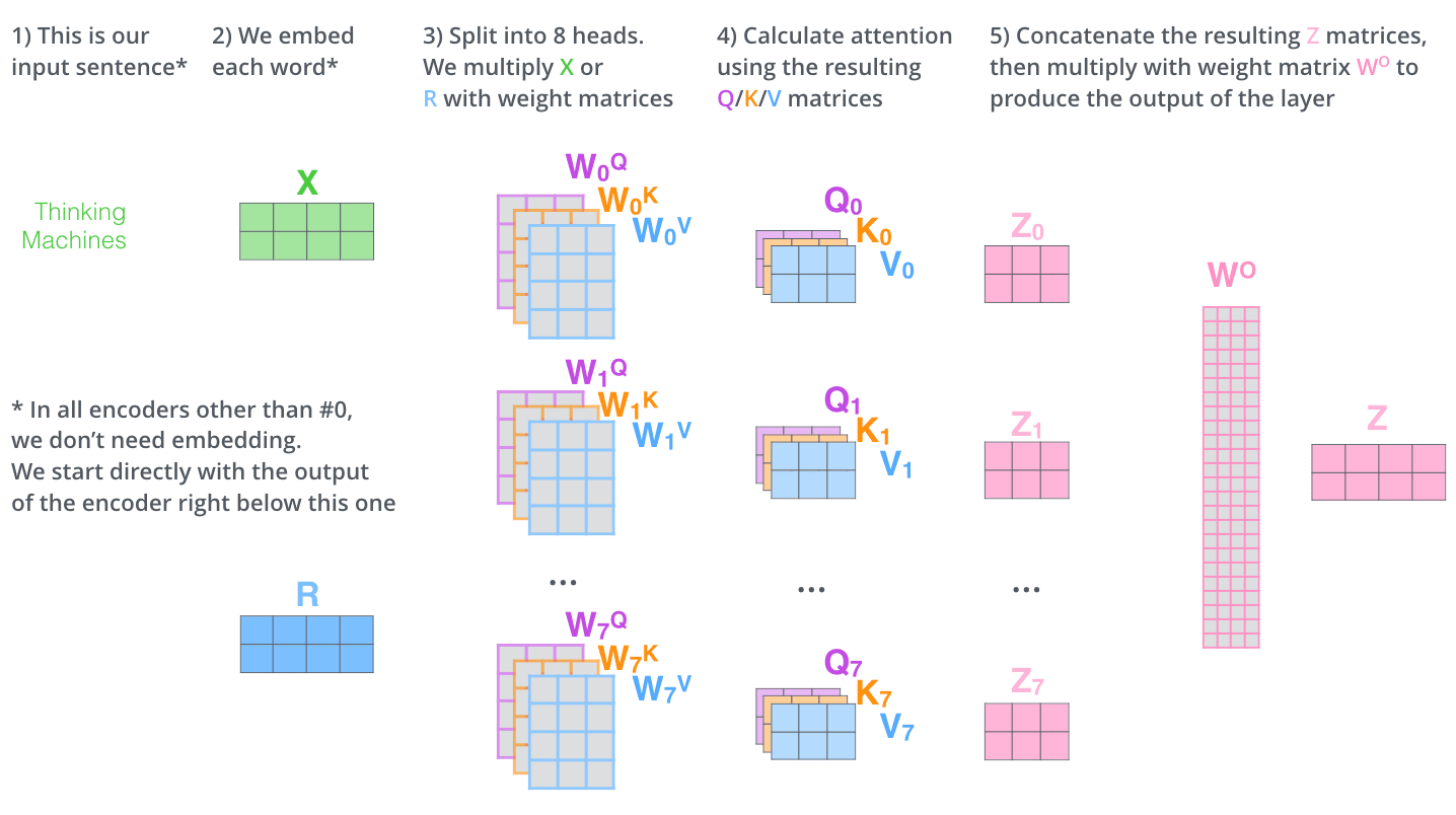
That’s pretty much all there is to multi-headed self-attention. It’s quite a handful of matrices, I realize. Let me try to put them all in one visual so we can look at them in one place

多头自注意力机制基本上就是这些。我意识到这里涉及很多矩阵。让我尝试将它们全部放在一个视觉中，这样我们就能在一个地方查看它们。

Now that we have touched upon attention heads, let’s revisit our example from before to see where the different attention heads are focusing as we encode the word “it” in our example sentence:

现在我们已经简要介绍了注意力头，让我们重新回顾之前的例子，看看在编码我们例句中的单词“it”时，不同的注意力头分别聚焦在哪里：

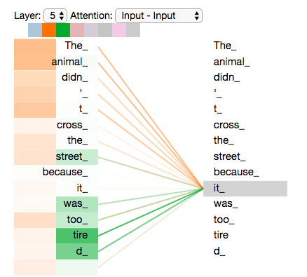
As we encode the word "it", one attention head is focusing most on "the animal", while another is focusing on "tired" -- in a sense, the model's representation of the word "it" bakes in some of the representation of both "animal" and "tired".

当我们编码单词"it"时，一个注意力头主要关注"the animal"，而另一个则关注"tired"——在某种意义上，模型对单词"it"的表征融入了"animal"和"tired"的部分表征。

If we add all the attention heads to the picture, however, things can be harder to interpret:

然而，如果我们把所有的注意力头都加到图片中，事情可能会变得难以解释：

Representing The Order of The Sequence Using Positional Encoding 使用位置编码表示序列的顺序

One thing that’s missing from the model as we have described it so far is a way to account for the order of the words in the input sequence.

到目前为止，我们所描述的模型中缺少的是一种方法来解释输入序列中单词的顺序。

To address this, the transformer adds a vector to each input embedding. These vectors follow a specific pattern that the model learns, which helps it determine the position of each word, or the distance between different words in the sequence. The intuition here is that adding these values to the embeddings provides meaningful distances between the embedding vectors once they’re projected into Q/K/V vectors and during dot-product attention.

为了解决这个问题，Transformer 为每个输入嵌入添加了一个向量。这些向量遵循模型学习的特定模式，这有助于它确定每个单词的位置，或序列中不同单词之间的距离。这里的直观理解是，将这些值添加到嵌入中，在它们被投影到 Q/K/V 向量并在点积注意力期间时，会提供有意义的嵌入向量之间的距离。

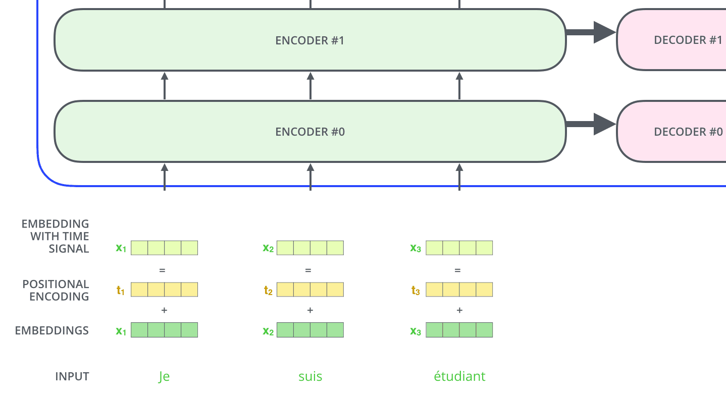
To give the model a sense of the order of the words, we add positional encoding vectors -- the values of which follow a specific pattern.

为了让模型感知到单词的顺序，我们添加了位置编码向量——这些向量的值遵循特定的模式。

If we assumed the embedding has a dimensionality of 4, the actual positional encodings would look like this:

如果我们假设嵌入的维度为 4，实际的位置编码将如下所示：

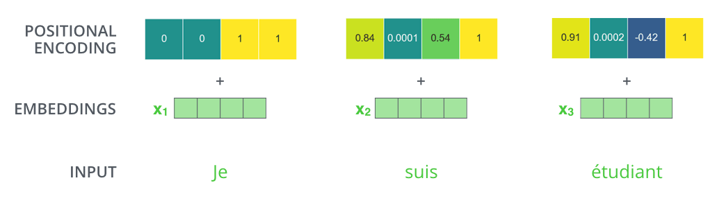
A real example of positional encoding with a toy embedding size of 4

一个使用玩具嵌入大小为 4 的真实位置编码示例

What might this pattern look like?

这种模式可能看起来像什么？

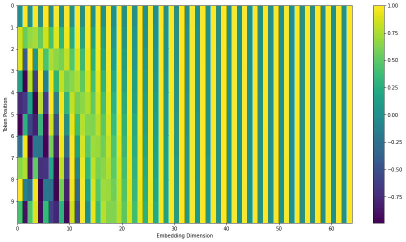
In the following figure, each row corresponds to a positional encoding of a vector. So the first row would be the vector we’d add to the embedding of the first word in an input sequence. Each row contains 512 values – each with a value between 1 and -1. We’ve color-coded them so the pattern is visible.

在下图中，每一行对应于一个向量的位置编码。因此，第一行将是我们在输入序列的第一个词的嵌入中要添加的向量。每一行包含 512 个值——每个值介于 1 和-1 之间。我们用颜色编码它们，以便模式可见。

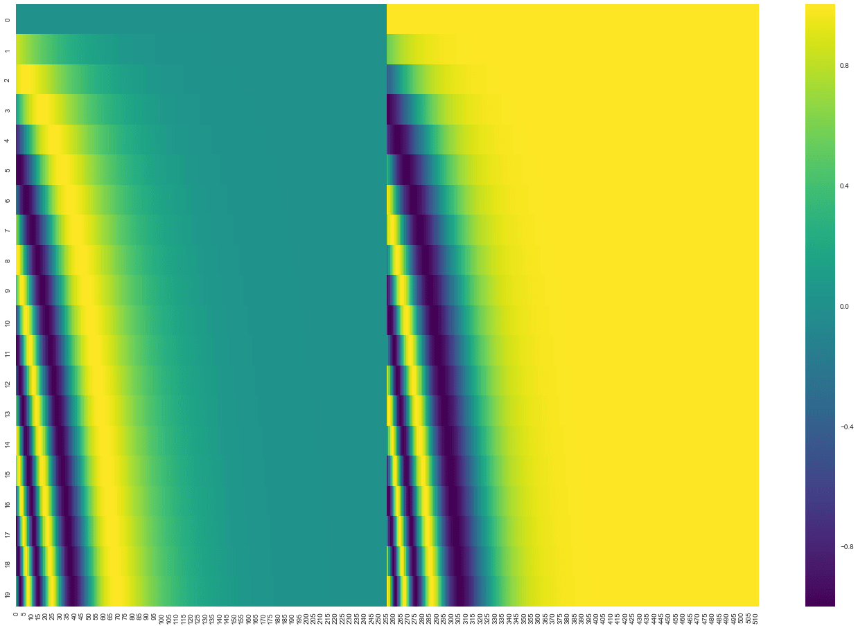
A real example of positional encoding for 20 words (rows) with an embedding size of 512 (columns). You can see that it appears split in half down the center. That's because the values of the left half are generated by one function (which uses sine), and the right half is generated by another function (which uses cosine). They're then concatenated to form each of the positional encoding vectors.

一个 20 个词（行）的 512 维（列）位置编码的真实示例。你可以看到它沿中心被分成两半。这是因为左半部分值由一个函数生成（该函数使用正弦），右半部分值由另一个函数生成（该函数使用余弦）。然后它们被连接起来形成每个位置编码向量。

The formula for positional encoding is described in the paper (section 3.5). You can see the code for generating positional encodings in get_timing_signal_1d(). This is not the only possible method for positional encoding. It, however, gives the advantage of being able to scale to unseen lengths of sequences (e.g. if our trained model is asked to translate a sentence longer than any of those in our training set).

位置编码的公式在论文中进行了描述（第 3.5 节）。生成位置编码的代码可以在 get_timing_signal_1d() 中找到。但这并不是位置编码的唯一可能方法。然而，它具有能够扩展到未见过的序列长度的优点（例如，如果我们的训练模型被要求翻译一个比训练集中任何句子都长的句子）。

July 2020 Update: The positional encoding shown above is from the Tensor2Tensor implementation of the Transformer. The method shown in the paper is slightly different in that it doesn’t directly concatenate, but interweaves the two signals. The following figure shows what that looks like. Here’s the code to generate it:

2020 年 7 月更新：上面展示的位置编码来自 Transformer 的 Tensor2Tensor 实现。论文中展示的方法略有不同，它不是直接拼接，而是交织这两种信号。下面的图展示了它看起来是怎样的。这是生成它的代码：

The Residuals 残差

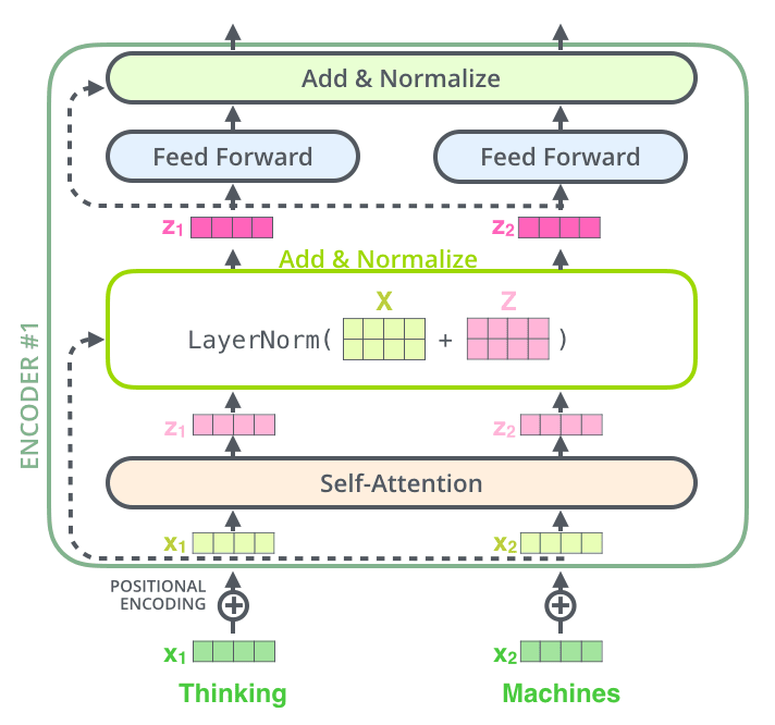
One detail in the architecture of the encoder that we need to mention before moving on, is that each sub-layer (self-attention, ffnn) in each encoder has a residual connection around it, and is followed by a layer-normalization step.

在继续之前，我们需要提及编码器架构中的一个细节：每个编码器中的每个子层（自注意力机制、前馈神经网络）都有一个残差连接，并且随后进行层归一化处理。

If we’re to visualize the vectors and the layer-norm operation associated with self attention, it would look like this:

如果我们想要可视化与自注意力相关的向量和层归一化操作，它看起来会像这样：

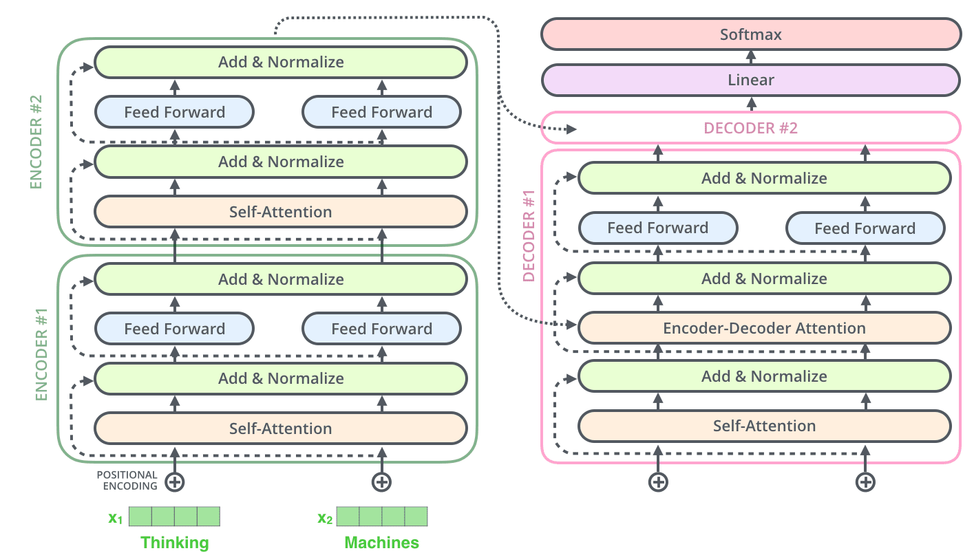
This goes for the sub-layers of the decoder as well. If we’re to think of a Transformer of 2 stacked encoders and decoders, it would look something like this:

这同样适用于解码器的子层。如果我们考虑一个由 2 个堆叠的编码器和解码器组成的 Transformer，它看起来会像这样：

The Decoder Side 解码器侧 Now that we’ve covered most of the concepts on the encoder side, we basically know how the components of decoders work as well. But let’s take a look at how they work together.

现在我们已经涵盖了编码器的大部分概念，基本上也知道了解码器各组件的工作方式。但让我们看看它们是如何协同工作的。

The encoder start by processing the input sequence. The output of the top encoder is then transformed into a set of attention vectors K and V. These are to be used by each decoder in its “encoder-decoder attention” layer which helps the decoder focus on appropriate places in the input sequence:

编码器首先处理输入序列。编码器顶层的输出随后被转换为一组注意力向量 K 和 V。这些向量将被每个解码器在其“编码器-解码器注意力”层中使用，帮助解码器专注于输入序列的适当位置：

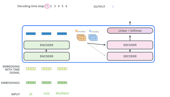
After finishing the encoding phase, we begin the decoding phase. Each step in the decoding phase outputs an element from the output sequence (the English translation sentence in this case).

编码阶段完成后，我们开始解码阶段。解码阶段的每一步都会输出输出序列中的一个元素（在这个例子中是英语翻译句子）。

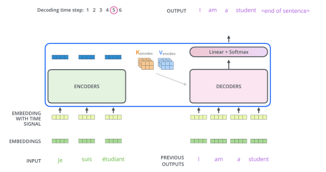
The following steps repeat the process until a special symbol is reached indicating the transformer decoder has completed its output. The output of each step is fed to the bottom decoder in the next time step, and the decoders bubble up their decoding results just like the encoders did. And just like we did with the encoder inputs, we embed and add positional encoding to those decoder inputs to indicate the position of each word.

以下步骤会重复执行，直到出现特殊符号，表明 Transformer 解码器已完成输出。每一步的输出会输入到下一个时间步的底部解码器中，解码器像编码器一样逐层传递它们的解码结果。与我们对编码器输入所做的一样，我们会对解码器输入进行嵌入并添加位置编码，以指示每个单词的位置

The self attention layers in the decoder operate in a slightly different way than the one in the encoder:

解码器中的自注意力层与编码器中的工作方式略有不同：

In the decoder, the self-attention layer is only allowed to attend to earlier positions in the output sequence. This is done by masking future positions (setting them to -inf) before the softmax step in the self-attention calculation.

在解码器中，自注意力层仅被允许关注输出序列中较早的位置。这是通过在自注意力计算中的 softmax 步骤之前对未来的位置进行掩码（将它们设置为 -inf ）来实现的。

The “Encoder-Decoder Attention” layer works just like multiheaded self-attention, except it creates its Queries matrix from the layer below it, and takes the Keys and Values matrix from the output of the encoder stack.

“编码器-解码器注意力”层的工作方式与多头自注意力类似，只是它从下层创建其查询矩阵，并从编码器堆栈的输出中获取键和值矩阵。

The Final Linear and Softmax Layer 最终线性层和 Softmax 层

The decoder stack outputs a vector of floats. How do we turn that into a word? That’s the job of the final Linear layer which is followed by a Softmax Layer.

解码器堆栈输出一个浮点数向量。我们如何将其转换为单词？这是最终线性层的工作，它后面跟着一个 Softmax 层。

The Linear layer is a simple fully connected neural network that projects the vector produced by the stack of decoders, into a much, much larger vector called a logits vector.

线性层是一个简单的全连接神经网络，它将解码器堆栈产生的向量投影到一个称为 logits 向量的、大得多的向量中。

Let’s assume that our model knows 10,000 unique English words (our model’s “output vocabulary”) that it’s learned from its training dataset. This would make the logits vector 10,000 cells wide – each cell corresponding to the score of a unique word. That is how we interpret the output of the model followed by the Linear layer.

假设我们的模型知道 10,000 个独特的英语单词（模型“输出词汇表”），这些单词是从其训练数据集中学到的。这将使 logits 向量有 10,000 个单元格宽——每个单元格对应一个独特单词的得分。这就是我们如何解释经过线性层后的模型输出。

The softmax layer then turns those scores into probabilities (all positive, all add up to 1.0). The cell with the highest probability is chosen, and the word associated with it is produced as the output for this time step.

然后，softmax 层将这些分数转换为概率（所有都是正数，总和为 1.0）。选择概率最高的单元，并将其关联的词作为该时间步的输出。

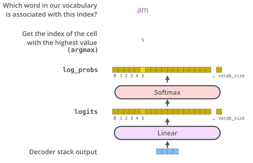
This figure starts from the bottom with the vector produced as the output of the decoder stack. It is then turned into an output word.

这个图从底部开始，以解码器堆栈产生的向量为输出。然后它被转换成一个输出词。

Recap Of Training 训练回顾

Now that we’ve covered the entire forward-pass process through a trained Transformer, it would be useful to glance at the intuition of training the model.

现在我们已经了解了通过训练好的 Transformer 进行整个前向传递过程，那么了解模型训练的直观概念将会有所帮助。

During training, an untrained model would go through the exact same forward pass. But since we are training it on a labeled training dataset, we can compare its output with the actual correct output.

在训练过程中，未训练的模型会经历完全相同的前向传递。但由于我们在标记的训练数据集上进行训练，我们可以将其输出与实际正确的输出进行比较。

To visualize this, let’s assume our output vocabulary only contains six words(“a”, “am”, “i”, “thanks”, “student”, and “” (short for ‘end of sentence’)).

为了可视化这一点，让我们假设我们的输出词汇表只包含六个词（“a”，“am”，“i”，“thanks”，“student”，以及“”（意为“句子结束”）。

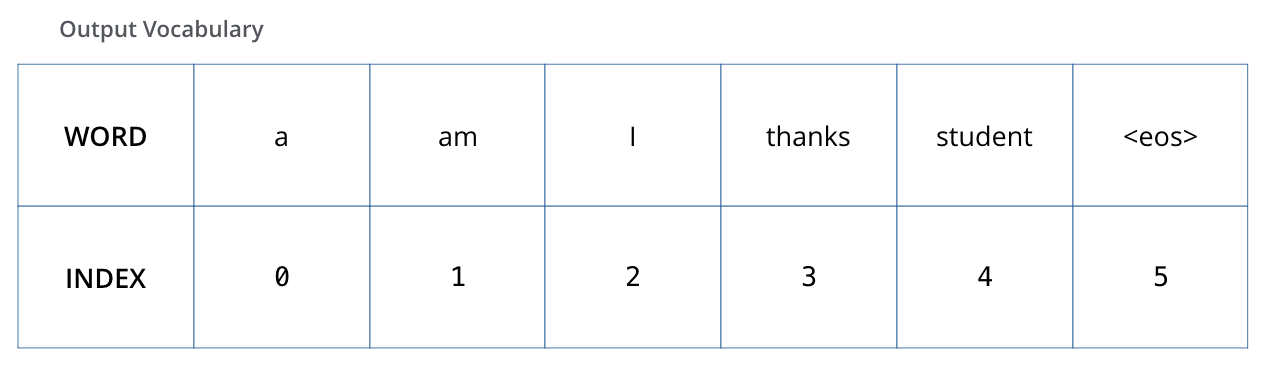
The output vocabulary of our model is created in the preprocessing phase before we even begin training.

我们的模型的输出词汇是在训练开始前的预处理阶段创建的。

Once we define our output vocabulary, we can use a vector of the same width to indicate each word in our vocabulary. This also known as one-hot encoding. So for example, we can indicate the word “am” using the following vector:

一旦我们定义了输出词汇表，就可以使用一个宽度相同的向量来表示词汇表中的每个词。这也被称为 one-hot 编码。例如，我们可以使用以下向量来表示单词“am”：

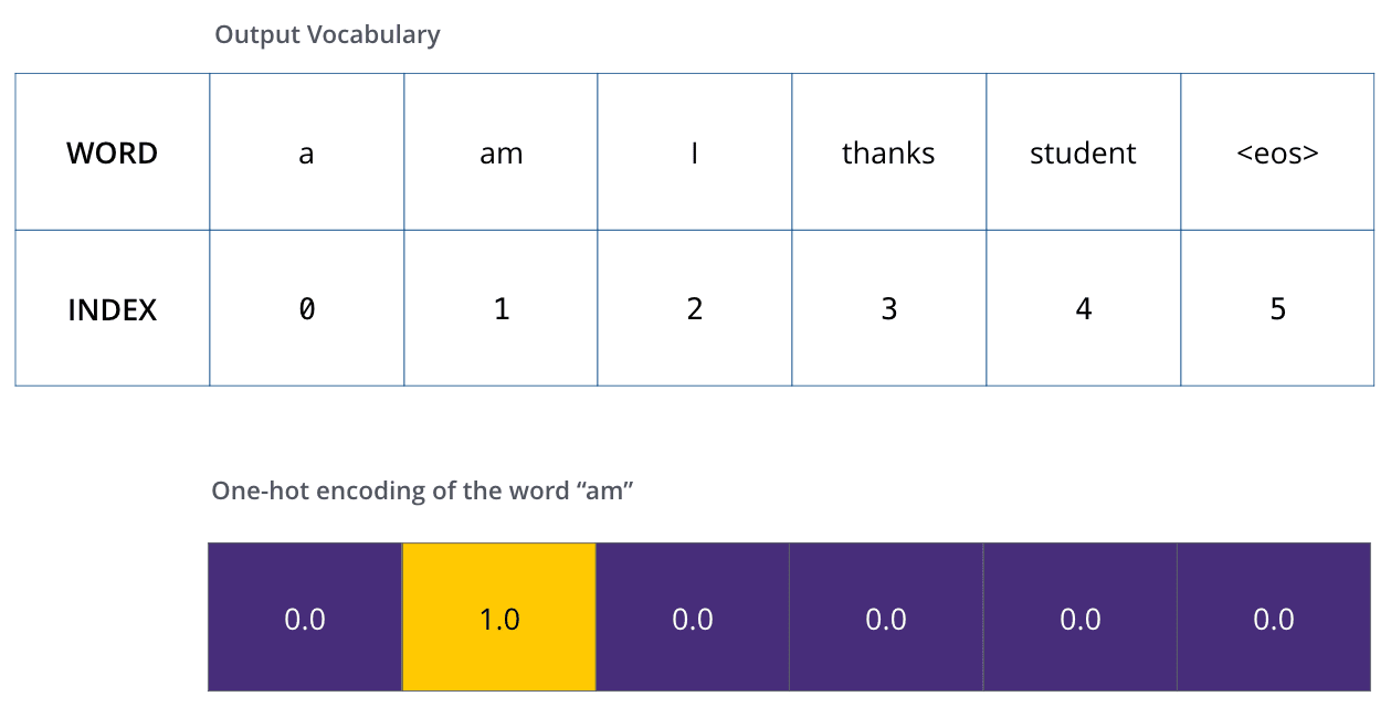
Example: one-hot encoding of our output vocabulary

示例：我们输出词汇表的一热编码

Following this recap, let’s discuss the model’s loss function – the metric we are optimizing during the training phase to lead up to a trained and hopefully amazingly accurate model.

在回顾之后，让我们来讨论模型的损失函数——这是我们在训练阶段优化的指标，目的是最终得到一个训练完成且希望非常准确的模型。

The Loss Function 损失函数

Say we are training our model. Say it’s our first step in the training phase, and we’re training it on a simple example – translating “merci” into “thanks”.

假设我们正在训练模型。假设这是训练阶段的第一步，我们正在用一个简单的例子来训练它——将“merci”翻译成“thanks”。

What this means, is that we want the output to be a probability distribution indicating the word “thanks”. But since this model is not yet trained, that’s unlikely to happen just yet.

这意味着，我们希望输出是一个概率分布，表明单词“thanks”。但由于这个模型尚未训练，目前还不太可能实现。

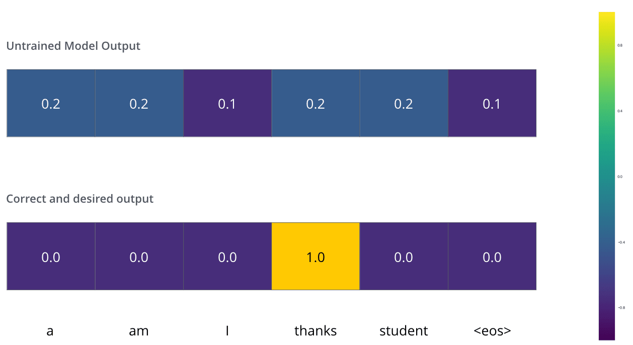
Since the model's parameters (weights) are all initialized randomly, the (untrained) model produces a probability distribution with arbitrary values for each cell/word. We can compare it with the actual output, then tweak all the model's weights using backpropagation to make the output closer to the desired output.

由于模型的参数（权重）都是随机初始化的，因此（未训练的）模型会为每个单元格/单词生成一个具有任意值的概率分布。我们可以将其与实际输出进行比较，然后使用反向传播调整模型的所有权重，使输出更接近期望的输出。

How do you compare two probability distributions? We simply subtract one from the other. For more details, look at cross-entropy and Kullback–Leibler divergence.

如何比较两个概率分布？我们只需将其中一个减去另一个。想了解更多细节，请查看交叉熵和 Kullback-Leibler 散度。

But note that this is an oversimplified example. More realistically, we’ll use a sentence longer than one word. For example – input: “je suis étudiant” and expected output: “i am a student”. What this really means, is that we want our model to successively output probability distributions where:

但请注意，这是一个过于简化的例子。更现实的情况是，我们会使用一个由多个单词组成的句子。例如——输入：“je suis étudiant”，预期输出：“i am a student”。这真正意味着，我们希望我们的模型能够依次输出概率分布，其中：

• Each probability distribution is represented by a vector of width vocab_size (6 in our toy example, but more realistically a number like 30,000 or 50,000)

• 每个概率分布由一个宽度为 vocab_size（在我们的玩具示例中是 6，但更现实的是一个像 30,000 或 50,000 的数字）的向量表示

• The first probability distribution has the highest probability at the cell associated with the word “i”

• 第一个概率分布在对应单词“i”的单元中具有最高概率

• The second probability distribution has the highest probability at the cell associated with the word “am”

• 第二个概率分布在对应单词“am”的单元中具有最高概率

• And so on, until the fifth output distribution indicates ‘’ symbol, which also has a cell associated with it from the 10,000 element vocabulary.

• 如此类推，直到第五个输出分布指示“ ”符号，该符号也与 10,000 元素词汇表中关联的一个单元相关联。

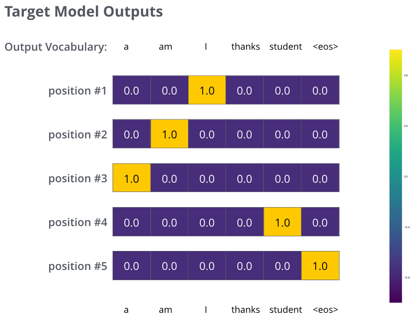
The targeted probability distributions we'll train our model against in the training example for one sample sentence.

在训练示例中，我们将针对一个样本句子训练模型的目标概率分布。

After training the model for enough time on a large enough dataset, we would hope the produced probability distributions would look like this:

在模型在足够大的数据集上训练足够长的时间后，我们希望产生的概率分布看起来是这样的：

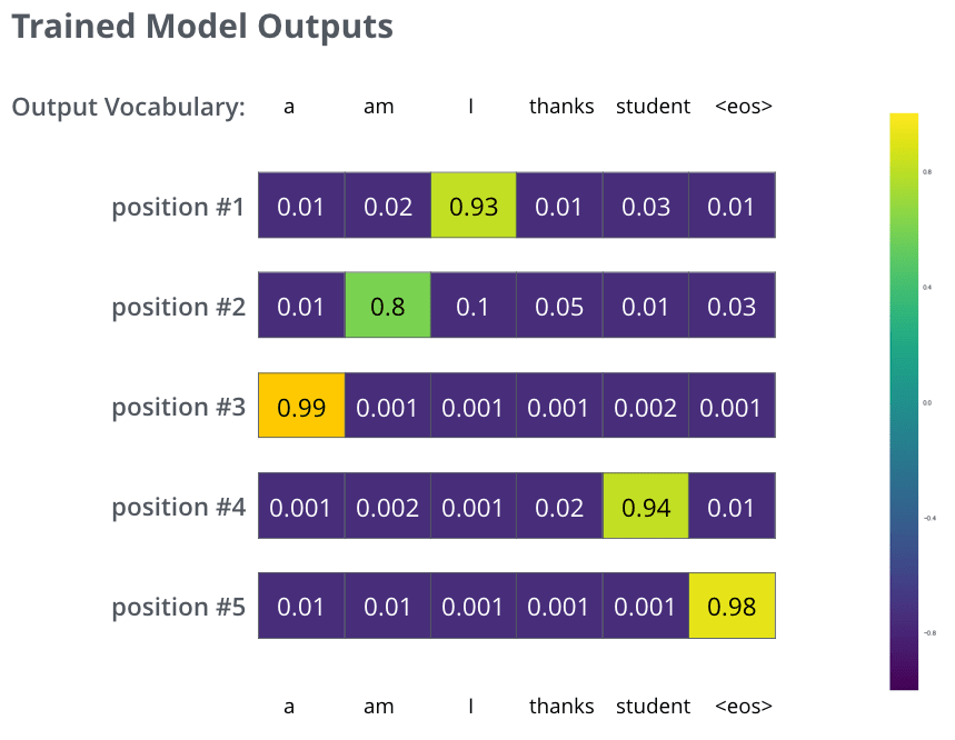
Hopefully upon training, the model would output the right translation we expect. Of course it's no real indication if this phrase was part of the training dataset (see: cross validation). Notice that every position gets a little bit of probability even if it's unlikely to be the output of that time step -- that's a very useful property of softmax which helps the training process.

希望经过训练后，模型能输出我们预期的正确翻译。当然，如果这个短语是训练数据集的一部分，这并不能真正说明问题（参见：交叉验证）。请注意，即使某个位置不太可能是该时间步的输出，它也会得到一定的概率——这是 softmax 的一个非常有用的特性，有助于训练过程。

Now, because the model produces the outputs one at a time, we can assume that the model is selecting the word with the highest probability from that probability distribution and throwing away the rest. That’s one way to do it (called greedy decoding). Another way to do it would be to hold on to, say, the top two words (say, ‘I’ and ‘a’ for example), then in the next step, run the model twice: once assuming the first output position was the word ‘I’, and another time assuming the first output position was the word ‘a’, and whichever version produced less error considering both positions #1 and #2 is kept. We repeat this for positions #2 and #3…etc. This method is called “beam search”, where in our example, beam_size was two (meaning that at all times, two partial hypotheses (unfinished translations) are kept in memory), and top_beams is also two (meaning we’ll return two translations). These are both hyperparameters that you can experiment with.

现在，由于模型一次生成一个输出，我们可以假设模型从概率分布中选择概率最高的词，并丢弃其余的词。这是其中一种方法（称为贪婪解码）。另一种方法是保留前两个词，比如“我”和“a”，然后在下一步中运行模型两次：一次假设第一个输出位置是“我”，另一次假设第一个输出位置是“a”，并选择在位置 1 和位置 2 都产生较少误差的版本。我们以此类推，对位置 2、位置 3 等进行处理。这种方法称为“束搜索”，在我们的例子中，束大小为 2（意味着在任何时候，内存中保留两个部分假设（未完成的翻译）），top_beams 也是 2（意味着我们将返回两个翻译）。这些都是可以实验的超参数。